Landsat 8 - pt.2

This blog post will cover progress I've recently made on some spatiotemporal tools to analyze and visualize Landsat 8 data.

Goals:

• Calculate the average land surface temperature (LST)  and normalized distribution vegetation index (NDVI) in a given location over time

• Calculate the change is LST and NDVI in a given location over time and identify what locations have seen the greatest positive and negative changes.

Process:

For this exercise I will be analyzing Landsat imagery of Lawrence Kansas, taken between 2013-2023. I will be using the Google Earth Engine to filter the imagery within the given date ranges (spanning from May-September of each year in the analysis period), generate simple composite imagery to remove cloud coverage and shadows, and will export the resulting imagery to Google drive, where I will download the files for local processing.  

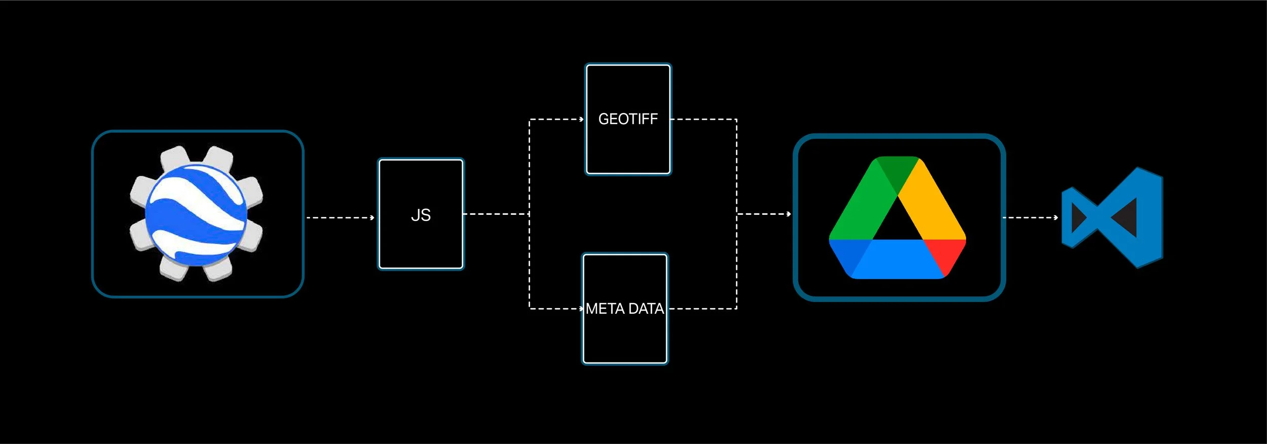
This diagram outlines a high level workflow, going from the Google Earth Engine to VSCode. Inside the Google Earth Engine, we use the JavaScript code editor to extract, filter and combine imagery and export it to Google Drive. We export the imagery as geoTiff (Geographic Tagged Image File Format) files. We also need to export the metadata of each geoTiff file which contain important information such as multipliers and constants used when calculating land surface temperature and other metrics. I exported this data as CSVs, but you can export them in whatever format best suits your workflow. Once the files are exported and saved to Google Drive, they can be downloaded and into your VSCode workspace for local processing. You can also process the files using cloud platforms like Google Colabs, but I prefer VSCode.

My VSCode workspace is organized into four main parts as shown in the diagram.

00_resources

• This folder contains reference files/datasets such as geospatial reference data which are referenced by one or more scripts in the "src" folder. Reference files in this folder include the following:

• zipcidesToGet.txt

• This file is referenced if we  want to break the main ROI extracted from the Google Earth Engine into smaller, sub ROIs. For example, if our main ROI encompasses a large city and we want to analyze data in  specific neighborhoods, we can enter the zip codes of those neighborhood into this file. A python script references this file and searches for the zip codes in a geographic reference file from the Census Bureau (ZCTA Gazzetteer) and returns the interpolated centers of the zip codes. The interpolated centers are then used to construct the sub-roi bounding boxes which are written to the roi.json file.

• roi.json

• This file contains the bounding box coordinates of the main ROI and the sub-ROIs. This file is referenced by multiple Python scripts during the aggregation and analysis process.

01_data

• This folder is the main storage space for data we want to analyze and contains the GeoTiff files exported from the Google Earth Engine as well as any additional data such as GIS parcel data. For this exercise we will not be going into the parcel analysis, but that is something I'm working.

02_output:

• This folder will contain pre-processed and analyzed data.

src

The src folder contains the source code for any data pre-processing, analysis and visualization. As of the time of writing this post, scripts in this folder include the following:

• poolBands.py

• This script reads geoTiff files in the 01_data folder and runs a pooling window (of a size determined by the user) over the imager that pools data from select bands in the multispectral imagery and calculates the mean of the data within the window. This process is used to reduce the amount of data to process in the temporal analysis by reducing the number of data points in the imagery. It's important to note that this process with reduce the detail of the output but will improve processing speed. The processed data for each GeoTiff file is written to individual JSON files with the same name as the GeoTiff. 

• normalizeLST.py

• This script reads the simplified imagery and normalizes land surface temperature data. This step is done so we can identify areas that have seen significant changes in thermal characteristics over time without being skewed by changes in weather from year to year.

• temporalAnalysis.py

  • This script reads the pooled and normalized landsat data and calculates changes in LST and NDVI over the analysis period. The script also references the roi.json file and used the bounding box of the main roi to construct real-world coordinates to map the analyzed data to. The resulting output is written to the temporal_analysis.json file in the 02_output folder.

Visualization

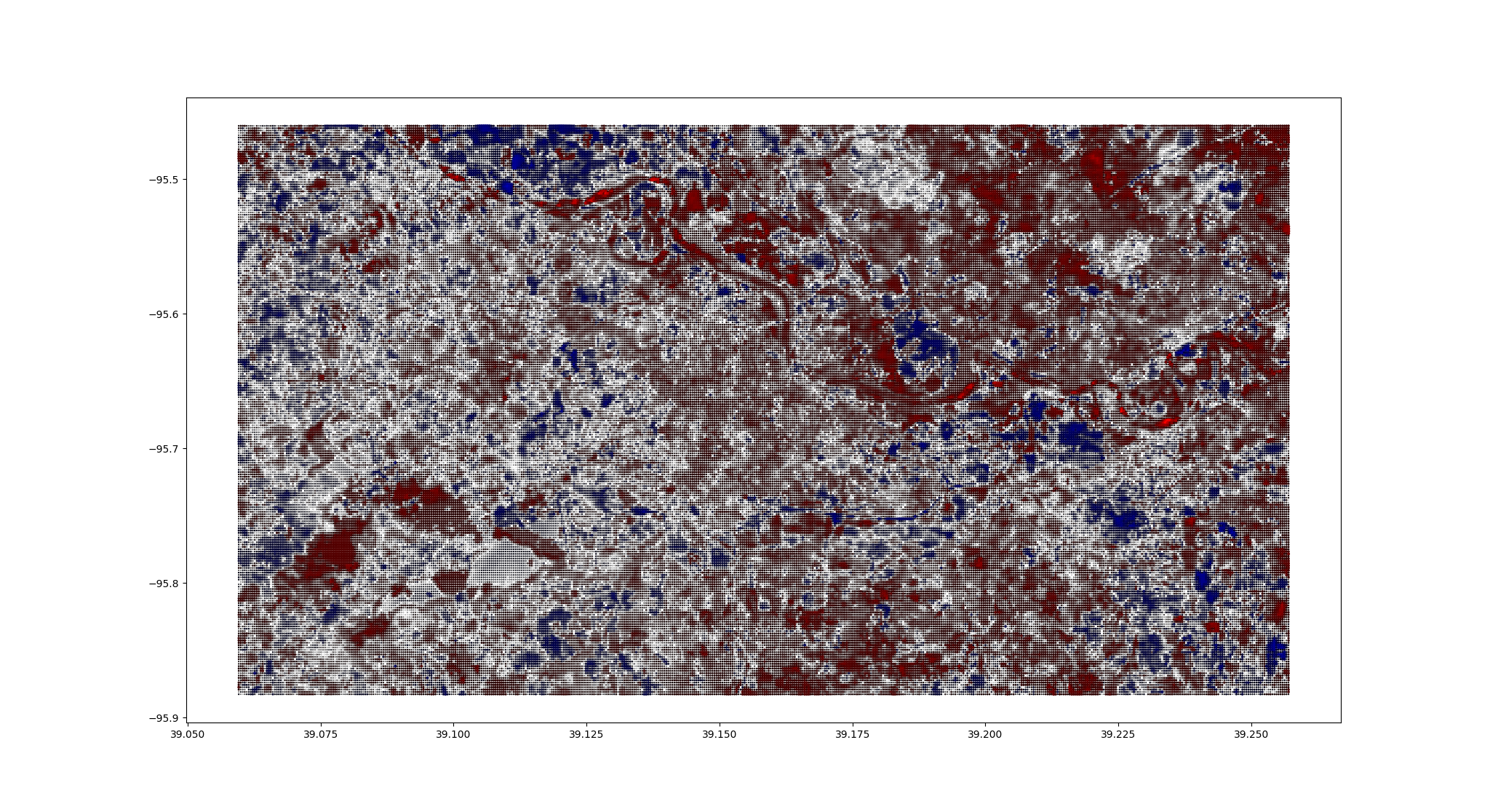
The following plots show the change in LST and NDVI over the analysis period. Red indicates a decrease in LST/NDVI and blue indicates an increase in LST/NDVI. The size and color intensity of the dot indicates the degree of change.

LST (Land Surface Temperature)

NDVI (Normalized Distribution Vegetation Index)

The following visualizations were experimentations made with Grasshopper to see how the temporally analyzed data would look when visualized in 3D. These examples show mean land surface temperatures using point clouds and polylines.