The U.S. federal government grants public access to a significant amount of data and many of my personal and professional projects utilize data from federal sources. This project was initially started as part of a research effort I was conducting for my job and I've decided to continue to develop the project on my personal. The aim of this project is to create a toolkit that helps people analyze and visualize government assistance and award contracts. This data is made available to the public on usaspending.gov where anyone can download datasets themselves. However, these datasets tend to be fairly large csv files, consisting of several hundred thousand rows and sometimes hundreds of columns depending on the agency. Additionally, like many datasets from government entities, data is often represented in the form of reference codes that correspond to reference tables. To analyze these datasets geospatially and to make sense of referential data requires one to combine several reference data tables and datasets together. Without proper tools to parse and analyze the data, these datasets are not useful. So with all that in mind I began developing a collection of computational tools to analyze and visualize these datasets. There are differences in the way data is structured and labeling systems used across difference government agencies, so these tools require some customization depending on which agencies' data you're working with. This example uses tools I made for working with datasets from the Department of Transportation. As I mentioned before, multiple data sources are required to make sense of these datasets, so we'll begin with an overview of each.

The Data

The DOT data itself can be access at usaspending.gov in the "Award Data Archive" section. This page allows you to select a specific agency and download federal assistance and contract datasets in csv format.

The dataset I downloaded for this example is for the 2023 fiscal year and consists of about 23000 rows (not bad) and 294 columns.

Much of the information in this file is not of particular interest to me, at least not for the purpose of this example, so we will instead focus on a select group of columns that contain the information we need to generate a relatively high level summary of the dataset.

To start, we want to know where these contracts are being awarded. To locate the geographic places where these federal dollars are going, we can use the following columns:

“primary_place_of_performance_state_code”

Data in this column gives us the two character abbreviation of the state e.g. WA, CA, TX…

“primary_place_of_performance_zip_4”

Data in this column gives us the nine character zipcode of the place where the federally funded project is/will be

It's important not to confuse these columns with "recipient_state_code" and "recipient_zip_4_code" as they indicate the state and zipcode of the contracted company involved, not the location of the project. This is also useful and relevant information if you want to know the location where a contracted company is registered but is outside the scope of this example.

Now that we have the zip codes of where these federally funded projects are, we need a way to find out where they are geographically. To do this we will use geographic reference files from the Census Bureau and a custom reference table. The Census Bureau provides access to Gazetteer files, which are used for geographically aggregating data and can be found here: https://www.census.gov/geographies/reference-files/time-series/geo/gazetteer-files.html. There are a variety of Gazetteer files, each of which serve as a reference lookup for tabulation areas and their interpolated geographic centers. For this project, we will want to use the zip code tabulation areas and the core base statistical area (CBSA) Gazetteer files.

Geographic Aggregation of Data

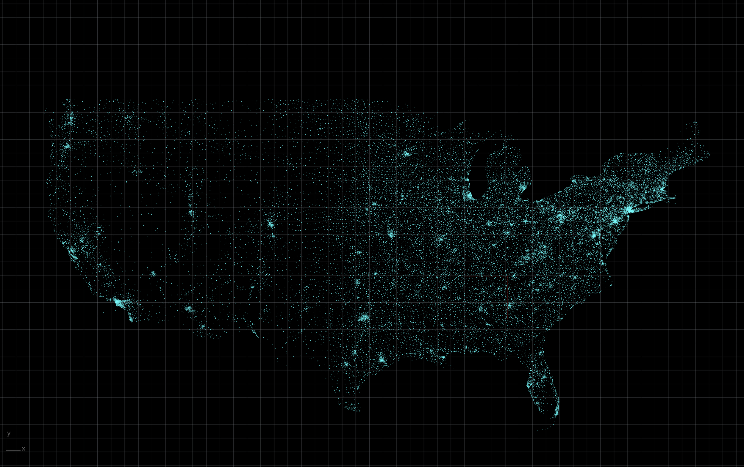
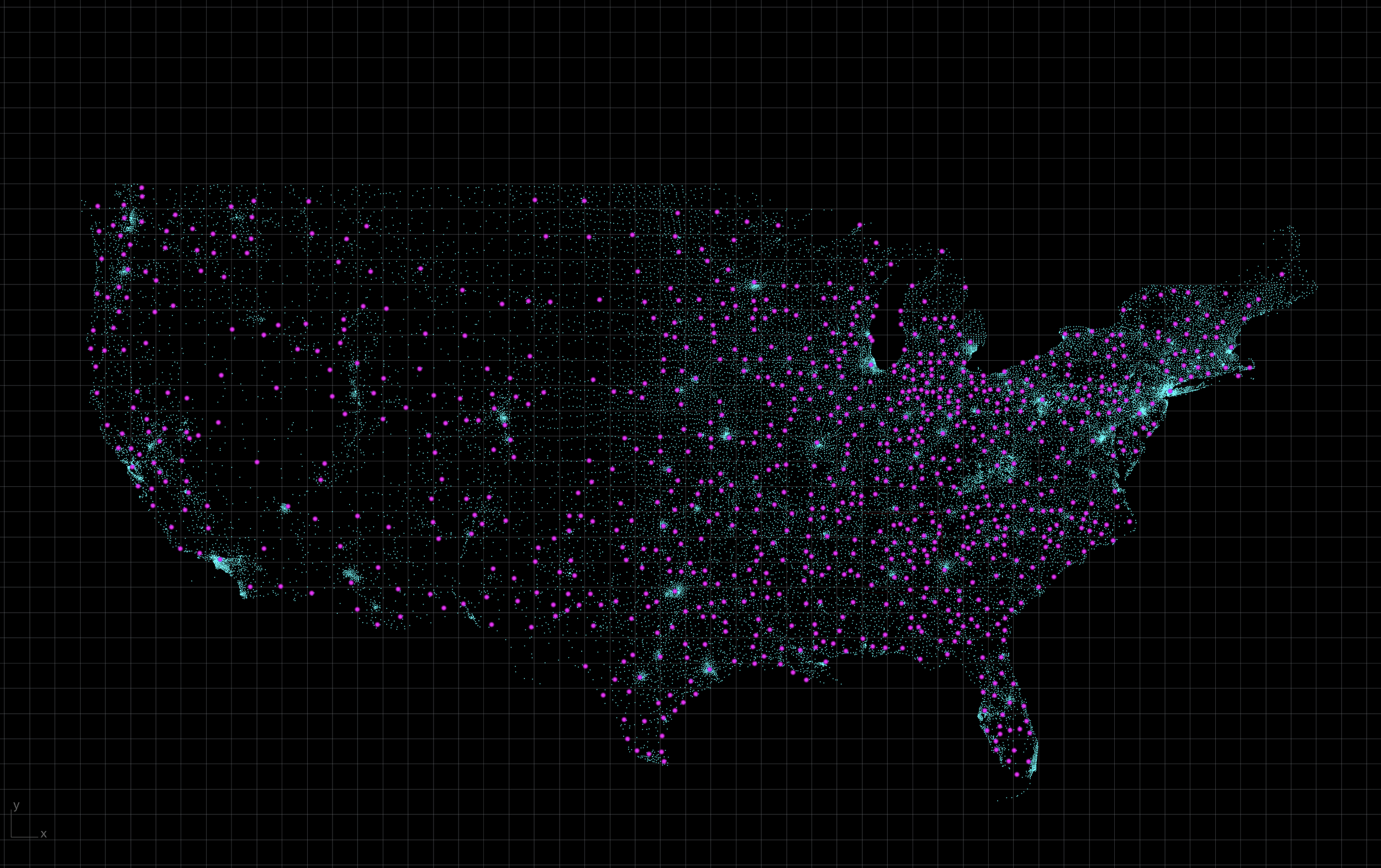
Given the U.S. has over 41,600 zipcodes, I set up these tools to aggregate contract data by CBSA. To do this, I wrote a custom geocrosswalk program that pools zipcodes with their respective CBSA and outputs an geocrosswalk.geoJson reference. I won't get into discussing to geocrosswalk program here, but I will in another post. In short, the geocrosswalk.geoJson reference file will allow us to easily lookup which CBSA a zipcode belongs to and we then associate the contract data with the CBSA. This way we are comparing a few hundred CBSAs instead of tens of thousands of individual zipcodes. However, the zipcode data is still kept in tact so we can filter by individual zipcodes if you wish to do so.

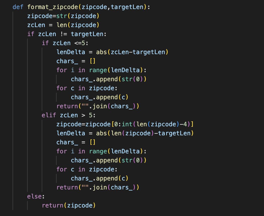
The zipcodes themselves require a bit of reformatting since the zipcode Gazetteer uses the five digit format whereas the DOT contract uses the nine digit format. The challenge here is that in csv format, zeros at the start of a zipcode are stripped in the dataset. So a zipcode such as "003456789" becomes "3456789". This complicates reformatting the zipcode because if the zipcide were kept with all its digits, we could simply partition the zipcode at the proper index and take the chunk we need. This problem is not overly complicated to fix but required writing this function (see below) to properly parse and format the zipcodes. Once the zipcode is formatted, we can search for it in the geocrosswalk and get its CBSA.

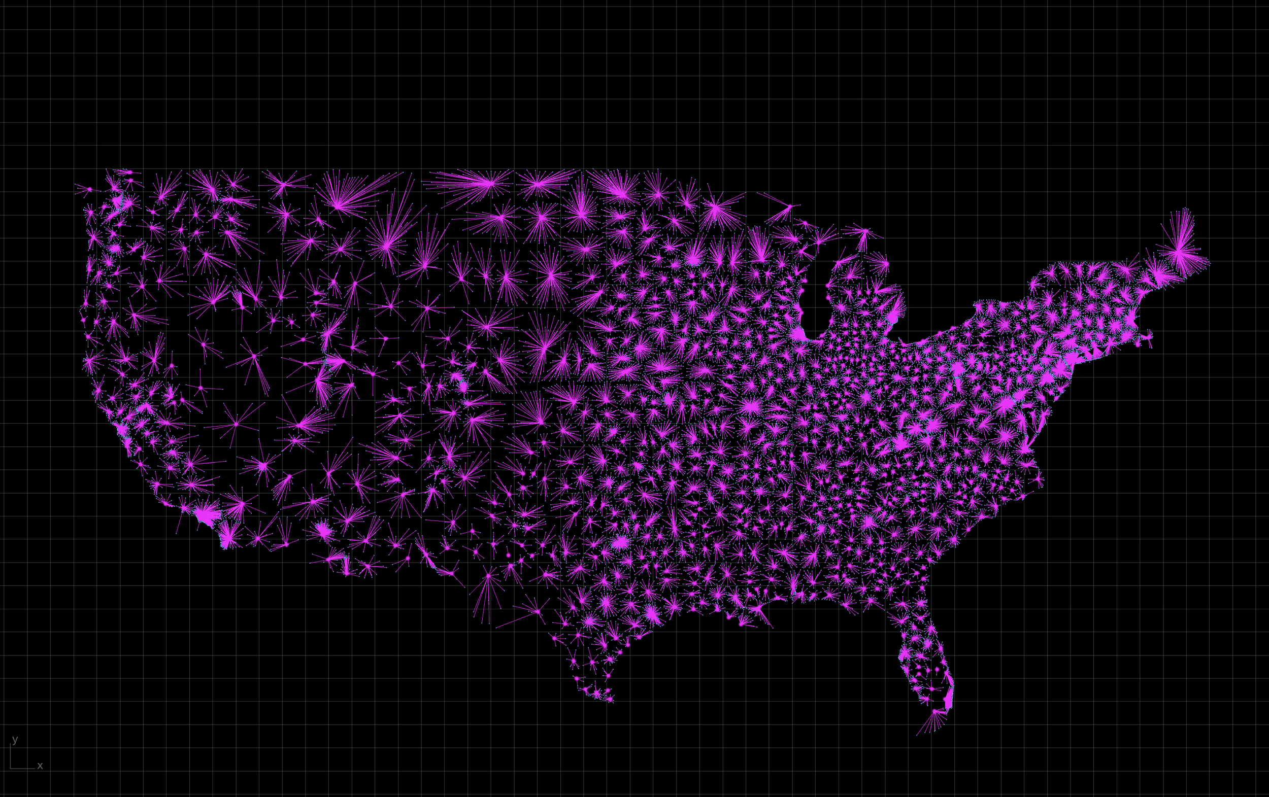
KNN - Nearest CBSA

To reduce the number of geographic to compare in the final output, contract data is aggregated with the nearest CBSA. This is simply calculated using a nearest neighbor algorithm and the results are written to geojson.

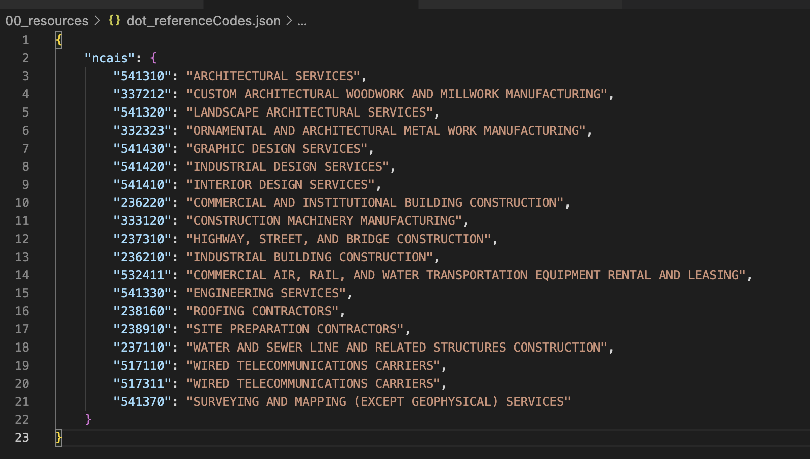
Another consideration that requires additional references is filtering the contract data by they type of contractor being awarded. These contract datasets contain awards on everything the agency is contracting, that includes big exciting infrastructure projects but it also contains information on perhaps less interesting contracts such as janitorial services. In order to filter out contracts we may not be interested in, we can use the NAICS code of the contract award recipient. NAICS stands for North American Industry Classification System and each prime contractor the federal government works with is given an NAICS designation based on they type of work they do. To select contract data for contracts related to industries we are interested in, we can reference another file that contains the NAICS codes. As the dataset is parsed through, if the NAICS code of the contractor does not appear in this file, the contract will be ignored.

The output

The output is written to csv and contains the following columns:

LOCID

This is the location id, in this case, the name of the core base statistical area that the contract data has been pooled with

LAT / LON

The interpolated center of the CBSA in latitude and longitude

STATE_CODE

A two character text abbreviation of the state

ZIPCODE

The zipcode from the "primary_place_of_performance_state_code" column

DIST

The geographic distance of the interpolated center of the zipcode to the interpolated center of the CBSA. This value is included to allow for filtering contract data by their distance away from the CBSA. This distance is calculated with the geocrosswalk program mentioned earlier which I will overview in another post.

FUND_TYPE

The type of fund. This information can be referenced here: https://www.acquisition.gov/far/part-16

NAICS_CODE

The NAICS code of the award recipient (the industry description by nature of work)

RECIPIENT

The official business name of the award recipient

ACTION_DATE

The date in which the contract was enacted

START_DATE

The date in which the project has or is expected to begin

END_DATE

The date in which the project has or is expected to end

PERMALINK

URL to the specific award data on USASpending.gov

FED_ATION_OBL

Any direct obligation of, or any obligation the full and timely payment of principal of and interest on which is guaranteed

CURRENT_TOTAL_VALUE

The total value of all funds to be allocated to the contract

SUBAGENCY

The name of the government subagency that awarded the contract. Eg. The FAA is a subagency of the Department of Transportation

DESCRIPTION

A brief text summary of the scope and nature of the project

For this example, I made a few quick visualizations with Kepler.GL that shows where federal dollars awarded by the Department of Transportation and its subagencies have been allocated. I’m currently working on making a variety of ways to interactively explore the the output with interactive visualizations made with d3js and Deck.GL (the graphics library that Kepler.GL is built with). I plan to post more about this project as I continue to develop it.

Analyzing Federal Spending - pt.1

The Data

Geographic Aggregation of Data

The output

Landsat 8 - pt.1

Image Characteristics with YOLOV8