Urban Change Analysis - Dynamic World V1

This post will overview an implementation of urban change analysis in Google Earth Engine using the Dynamic World V1 dataset and Sentinel-2 L1C image collection. Dynamic world is a near-real-time (NRT) land use/land cover (LULC) dataset. The dataset includes class probabilities and label information for nine classes. The nine classes include water, trees, grass, flooded_vegetation, crops, shrub_and_scrub, built, bare and snow_and_ice. The dataset is considered near-real-time due to the short revisit time of Sentinel-2 of about 2-5 days.  

The aim of this analysis is to identify where urban development has occurred in a given area over a specified window of time. The Sentinel-2 L1C image collection dates back to June 2015.

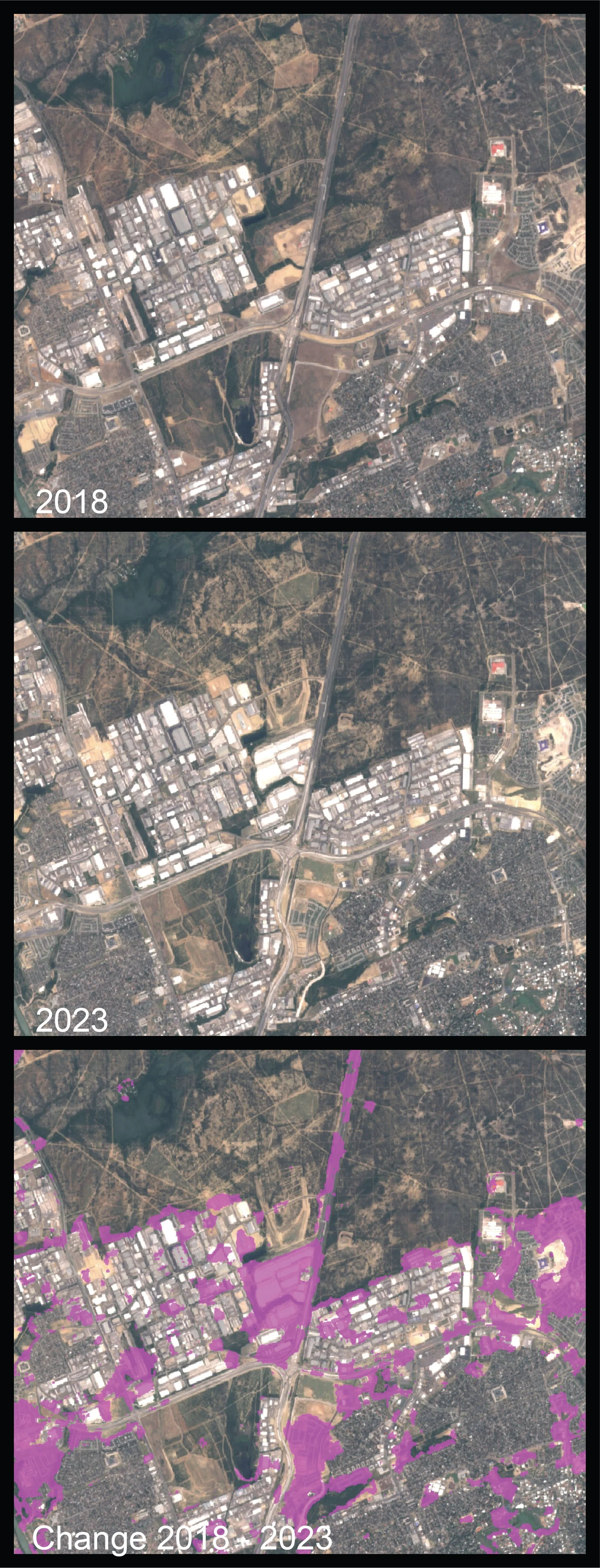
For this implementation, I used the JavaScript editor in Google Earth Engine and ran the analysis on the city of Laredo TX/Nuevo Laredo Mexico from 2018 through 2023.

Laredo is a primary port of entry between Mexico and the United States and is a major hub for the transportation of goods. Over the past few years, since the Covid-19 pandemic, we've seen significant changes to supply chains to improve resiliency. Laredo therefore seemed to be an interesting case study to test out this urban change analysis tool under the hypothesis that we would see a significant addition of warehousing facilities over the designated window of time.

The Code

The code for this implementation is very simple and consists of only 25 line of active JavaScript which can be seen below.

// Urban Growth Change Detection using Dynamic World Probability Bands
var expport = false;

var geom = geometry;
//Map.centerObject(geometry);

// Define the before and after time periods.
var beforeYear = 2018;
var afterYear = 2019;

// Create start and end dates for the before and after periods.
var beforeStart = ee.Date.fromYMD(beforeYear, 1 , 1);
var beforeEnd = beforeStart.advance(1, 'year');

var afterStart = ee.Date.fromYMD(afterYear, 1 , 1);
var afterEnd = afterStart.advance(1, 'year');

// Load the Dynamic World collection
var dw = ee.ImageCollection('GOOGLE/DYNAMICWORLD/V1')

// Filter the collection and select the 'built' band.
var dwFiltered = dw
  .filter(ee.Filter.bounds(geom))
  .select('built');

// Create mean composites
var beforeDw = dwFiltered.filter(
  ee.Filter.date(beforeStart, beforeEnd)).mean();
  
var afterDw = dwFiltered.filter(
  ee.Filter.date(afterStart, afterEnd)).mean();


// Add Sentinel-2 Composites to verify the results.
var s2 = ee.ImageCollection('COPERNICUS/S2_HARMONIZED')
     .filterBounds(geometry)
     .filter(ee.Filter.lt('CLOUDY_PIXEL_PERCENTAGE', 35));

// Create a median composite from sentinel-2 images.
var beforeS2 = s2.filterDate(beforeStart, beforeEnd).median();
var afterS2 = s2.filterDate(afterStart, afterEnd).median();
  
// Visualize images
var s2VisParams = {bands: ['B4', 'B3', 'B2'], min: 0, max: 3000};
Map.centerObject(geometry, 10);
Map.addLayer(beforeS2.clip(geom), s2VisParams, 'Before S2');
Map.addLayer(afterS2.clip(geom), s2VisParams, 'After S2');

// Select all pixels that have experienced large change
// in 'built' probbility
var builtChangeThreshold = 0.05; 
var newUrban = afterDw.subtract(beforeDw).gt(builtChangeThreshold);

var changeVisParams = {min: 0, max: 1, palette: ['white', '#ff23f8']};
Map.addLayer(newUrban.clip(geom), changeVisParams, 'New Urban');

// Mask all pixels with 0 value using selfMask()
var newUrbanMasked = newUrban.selfMask();

Map.addLayer(
  newUrbanMasked.clip(geom), changeVisParams, 'New Urban (Masked)');

// To ensure the masked values are set to NoData, 
// we cast the image to float and clip to geomery
var newUrbanMaskedExport = newUrbanMasked.toFloat().clip(geometry);

Results

The script was run a total of six times for various time increments. The first run we look at urban material change between imagery form 2018 and 2023 to show the overall difference across the full time window. Then, we can look at year to year changes between 2018-2019, 2019-2020, 2020-2021, 2021-2022 and 2022-2023. Areas that have seen change in urban materials (built structures) appear in magenta masked regions.

Overall change between 2018 - 2023.