2D to 3D Image Transform
The aim of this project has been to develop an efficient method to segment color images such that the output can be used for tracing and rudimentary construction in 3d space. The intention behind this project is to build the computational processes into a tool which can be used to quickly trace two-dimensional images, diagrams, maps, sketches etc. and import the segmented output into 3d design software like Rhino, where segmented pixel groups are treated as unique model elements. The value of this tool would be in reducing the time and labor involved in manually tracing images and to promote a more fluid connection in the design process between developing ideas by hand vs by software.
Palletization
A core component of this segmentation project is to separate the image into distinct layers based on color value. In order to reduce the computational load of later steps and to ensure image layers contained enough data points to make accurate feature calculations and grouping assignments, the image is first palletized to reduce the complexity of the image. This process is executed by iterating over the image with a slider 3X3 pixel slider window, which extracts the RGBA data from pixels within the pooling window and averages the color to yield the mean RGB (let's call this MC for "mean color") value of the pixels. MC is then referenced against an RGB space model which contains a collection of class objects that represent each color layer of the image. The distance is from MC to each color object is tested and if the MC is greater than a given distance threshold to its closest neighbor MC is added to the collection of color objects in the model. If the distance between MC and its closest neighbor is less than the given distance threshold, MC is not added to the model and pixels represented by MC are added to the closet neighboring color layer object. This step is done in order to simplify the color complexity of the image. The RGB space mode starts off empty and colors are added only if they are different enough from any existing color layers to be considered distinct. A lower distance threshold will result in more color layers whereas a higher distance threshold will result in fewer color layers.

Feature Extraction
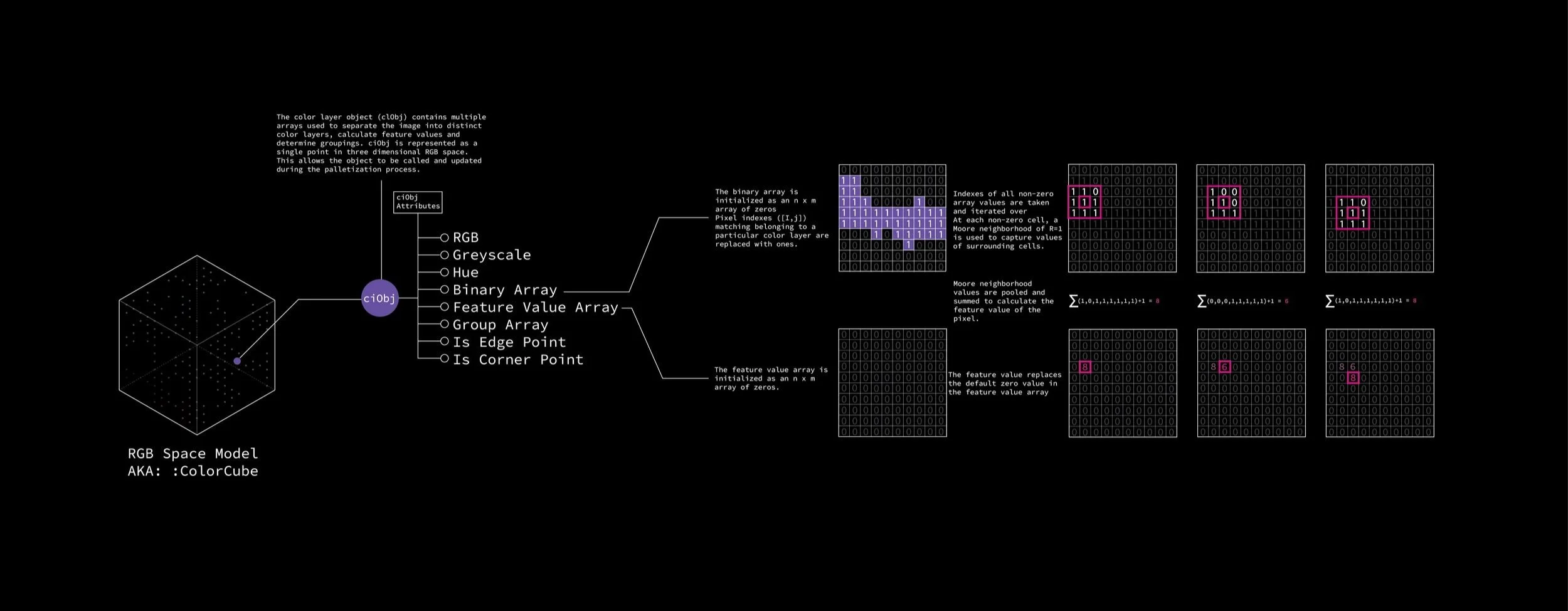
This step is used to classify cells by performing simple calculations that determines the cells relationship to neighboring cells. For example, is the cell an edge, a corner or part of a fill region?
To perform this step, each cell with non-zero value in the binary array a color layer is iterated over and the surrounding cells (Moore neighborhood of R=1) are looked at as well. A function returns the binary values of the surrounding cells and uses the binary value to determine how many adjacent cells belong to the same color layer.
After the cells are labeled with a feature value, we can select cells within the color layer matching specific feature values. To begin the cell grouping process, we begin by selecting cells with feature values of “9” because that indicates the cell is part of a fill region and surrounded by cells of the same palletized color on all sides and we can therefore make the greatest assumptions when applying group IDs (if most of the neighboring cells are of the same group, add the cell to their group).

Layering
As mentioned in the palletization section, the image is separated into distinct layers based on color values. Each layer consists of a class object with the following attributes.
ID: A unique ID to identify the layer based on its palletized color value
Binary pixel array: A 2d (n+2 X m+2) where n and m represent the size of the image with a single layer of padding. The binary array starts off with all values set to zero. If a pixel is allocated to the color object, the zero at the same index is set to 1. This results in a 2d array of ones and zeros where one indicates a pixel belonging to the color object exists at that index and zero means the pixel at that index does not belong to the color object.
Feature array: The feature is similar to the binary array in that all values are set to zero at the time the object is initialized. As feature values are calculated, the zero is replaced with a single digit value between 1 to 9. This process will be expanded on later.
Group array: You guessed it, this array is initialized the same way the two preceding arrays are. This array will contain unique group IDs for pixels as they are separated into distinct groups.
